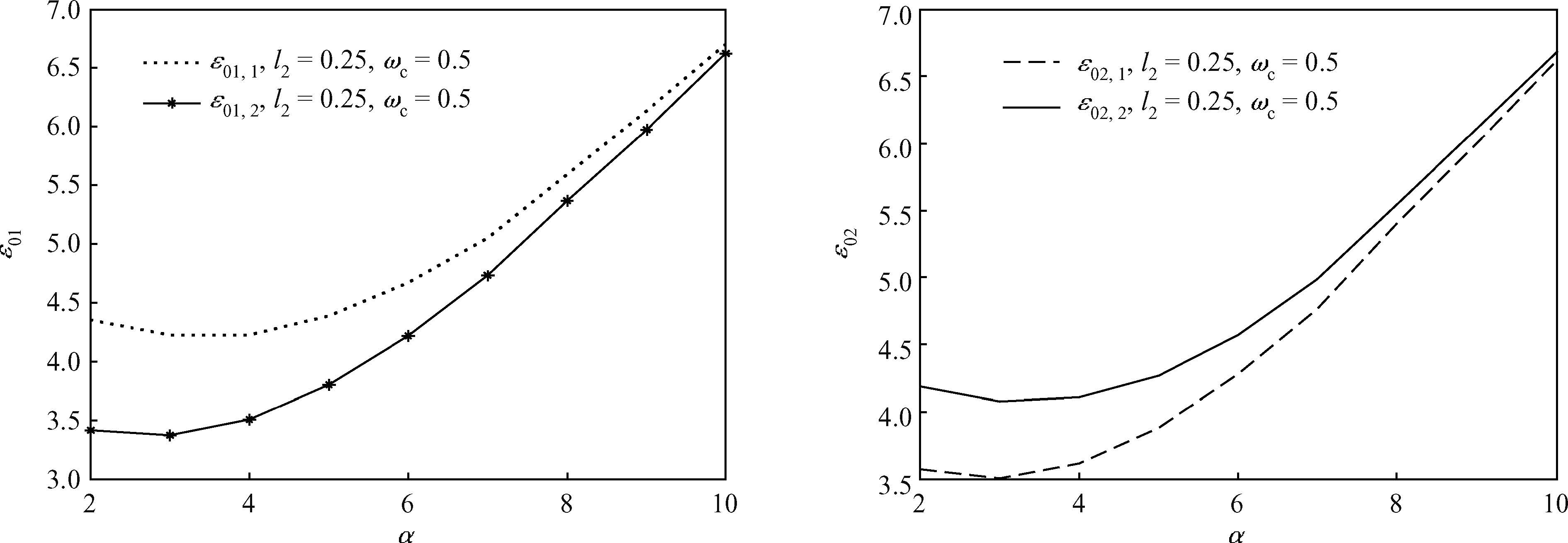
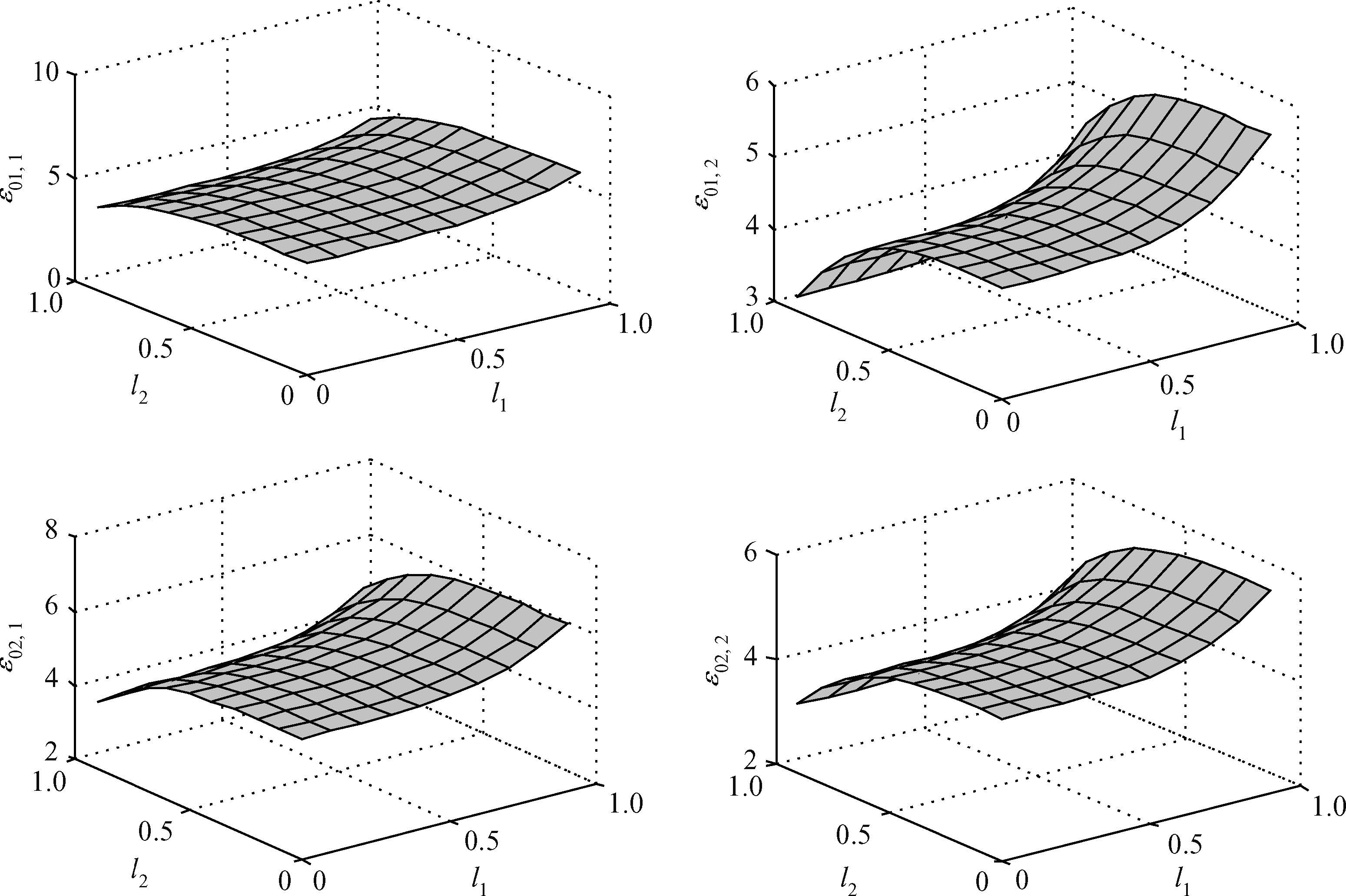
1. Introduction

Due to recent progress achieved in nanotechnology,it has become possible to fabricate low dimensional semiconductor structures. Special interest is being devoted to quasi zero dimensional structures,usually referred to as quantum dots (QDs)^{[1, 2, 3, 4, 5, 6, 7, 8, 9]}.In such nanometer QDs,some novel physical phenomena and potential electronic device applications have generated a great deal of interest. For example,computers based on quantum mechanics have proven to be more efficient in some specific calculations than those based on classical physics. The first step to build a quantum computer is the realization of the building block called a quantum bit (qubit) within the last decade. Various schemes have been proposed and many of them have even been realized^{[10, 11, 12]}. Among them,the most feasible approach is the quantum dot,because of its advantage of being integrated. Also,the large amount of experimental work on the quantum dot^{[13, 14, 15, 16, 17, 18]} is proof that the development of optoelectronic devices based on nanostructures prepared by colloidal chemical routes called quantum dots^[19] has attracted scientific and technological interest^{[20, 21, 22]}. This interest has been aroused because of their size and shape dependent electronic structure^{[23, 24]},their fluorescence emission is highly tunable^[25],their emission is linearly polarized ^[24],and because of their stimulated emission^[26]. Since Peng \textit{et al}.^[19],extensive development in the synthesis of colloidal QD has led to the possibility to synthesizing high-quality semiconductor nanoparticles capped by organic molecules and/or inorganic shells^{[25, 27]},which are easily processed via spin coating,self-assembling,and other low cost coating techniques currently used for device preparation. This may give theoretical physicists a considerable challenge to develop theory based on the quantum mechanical regime. Recently,much effort^{[28, 29, 30]} has been focused on exploring the polaron effect of QDs. Roussignol \textit{et al}.^[28] have shown experimentally and explained theoretically that phonon broadening is very significant in very small semiconductor QDs. Some have also observed[20,\,30] that the polaron effect is more important if the dot sizes are reduced to a few nanometers. More recently,the related problem of an optical polaron bound to a Coulomb impurity in a QD has also been considered in the presence of a magnetic field. Theoretical investigation of the polaron properties has been performed using the standard perturbation techniques^[31],by the variational Lee-Low-Pines (LLP) method^{[32, 33]},the modified LLP approach^{[34, 35]},the Feynman path integral method^[36],numerical diagonalization^[37],or Green function methods^[38]. The experimental data^[39] show,in particular,a large splitting width near the one-phonon and two-phonon resonances in a InAs/GaAs QD. This was accounted for by the theoretical model via a numerical diagonalization of the Fr\"{o}hlich interaction^[37]. The required value of the Fr\"{o}hlich constant was much larger (by a factor of two^[37]})$ than measured in bulk. In Reference ^[36] using the Feynman path integral method,the authors observed that the quadratic dependence of the magnetopolaron energy is modulated by a logarithmic function and strongly depends on the Fr\"{o}hlich electron-phonon coupling constant structure and cyclotron radius. Furthermore,the effective electron-phonon coupling is enhanced by high confinement or high magnetic field. In Reference ^[39] the polaron energy in QD was calculated using an LLP approach and it was found that the polaronic effect is more pronounced for small dot sizes. In Reference ^[34],using a modified LLP approach,the number of phonons around the electron,and the size of the polaron for the ground state,and for the first two excited states is calculated via the adiabatic approach. It is important to note that all of the previous studies do not taking into account the fact that the presence of magnetic field induces the interaction of the electron with the magnetic field and the procession of this electron along the $z$-axis. It is also instructive from the studies presented above to recall that polarons are often classified according to the Fröhlich electron-phonon coupling constant. The Feynman path integral method^[36] has been seen as one of the best methods because it simultaneously recovers all of the coupling types characterizing the Fröhlich electron-phonon coupling. The main feature of the method presented here is the modification of the LLP approach^[34] by the introduction of two new parameters,$b_1$ and $b_2$,which permits us to obtain an ``all coupling'' polaron theory. Here the coupling is weak if $b_1$ $=$ $b_2 =1$,strong coupling if $b_1 =b_2 =0$ and intermediate between these ranges.

In this work,we study the influence of the magnetic field and total momentum on the polaron ground state energy. In Section 2,we describe the model and the Hamiltonian of the system,and point out that this Hamiltonian will be explicitly dependent on the Zeeman effect. In Section 3 the analytical results of the ground state energy and of the polaron effective mass are obtained. In Section 4,we present a brief discussion of our results and finally we end with the conclusion.

2.Theory and calculation

The model that we use consists of an electron confined in an isotropic potential box with tunable dimensions immersed in a field of the bulk longitudinal optical (LO)-phonon modes,and interacting with an external magnetic field and the total momentum in $z$-direction. The dimensionless Hamiltonian describing the problem in Fröhlich units is given by^[40]

$\begin{equation} \label{eq1} H=H_{\rm e} +H_{\rm ph} +H_{\rm e-ph} , \end{equation}$

(1)

where $H_{\rm e}$ represents the electronic Hamiltonian and is given by

$\begin{equation} \label{eq2} H_{\rm e} =\frac{\boldsymbol{p}^2}{2m}+\frac{1}{2}m\Omega ^2\rho ^2+\frac{1}{2}m\omega _2 ^2z^2+\mu _{\rm B} B_{\rm ext} g_{\rm J} m_{\rm J}, \end{equation}$

(2)

where $\boldsymbol{p}$ is the momentum,$\omega _1$ and $\omega _2$ measure the confinement in the $xy$-plane and $z$-direction,respectively,and $\Omega ^2=\omega _1^2 +\omega _{\rm C}^2$. The fourth term of the Hamiltonian is the interaction of the magnetic moment with the total angular momentum $\omega _1^2$,where $\mu _{\rm B}$ is the Bohr magneton,$g_{\rm J}$ is the Land\'{e} $g$ factor,$m_{\rm J}$ is the magnetic total angular momentum numbers range from $-J$ to $\omega_1^2$. The Land\'{e} factor is giving by $g_{\rm J} =\frac{3}{2}+\frac{S(S+1)-L(L+1)}{2J(J+1)}$ ; $S$ is the spin and $L$ is the angular momentum.

$H_{\rm ph}$ is the phonon Hamiltonian defined as

$\begin{equation} \label{eq3} H_{\rm ph} =\sum\limits_Q {a_Q^+ a_Q } , \end{equation}$

(3)

where $a_Q^+$ $(a_Q)$ are the creation (annihilation) operators for LO phonons of wave vector $\boldsymbol{Q}=(q,q_z )$.

$H_{\rm e-ph}$ represents the electron-phonon Hamiltonian and is given by

$\begin{equation} \label{eq4} H_{\rm e-ph} =\sum\limits_Q {V_Q } \left[{a_Q {\rm e}^{{\rm i}Q.r}+a_Q^+ {\rm e}^{-{\rm i}Q.r}} \right], \end{equation}$

(4)

and $V_{Q}$ and $\alpha$ is the amplitude of the electron-phonon interaction and the coupling constant,respectively,given by

$\begin{equation} \label{eq5} \begin{split} {}& V_{q} ={\rm i}\left( {\frac{\hbar \omega _{\rm LO} }{q}} \right)\left( {\frac{\hbar }{2m\omega _{\rm LO} }} \right)^{1/4} \left( {\frac{4\pi \alpha }{V}} \right)^{1/2}, \\[2mm]& \alpha =\left( {\frac{e^2}{2\hbar \omega _{\rm LO} }} \right)\left( {\frac{2m\omega _{\rm LO} }{\hbar }} \right)^{1/2} \left( {\frac{1}{\varepsilon _\infty }-\frac{1}{\varepsilon _0 }} \right)^{1/2}. \\ \end{split} \end{equation}$

(5)

3.Ground state energy

Adopting the mixed-coupling approximation of Reference ^[41],we propose a modification to the first LLP-transformation by inserting two variational parameters,$b_1$ and $b_2$.

Our new unitary transformation is now^[35]

$\begin{equation} \label{eq6} U_1 =\exp \left\{{{\rm i}\left[{(\boldsymbol{P}_\rho -\boldsymbol{P}_\rho )\boldsymbol{\rho}b_1 +(P_z -P_\rho )zb_2 } \right]} \right\}, \end{equation}$

(6)

with

$\begin{equation} \label{eq7} \boldsymbol{P}=\boldsymbol{p}+\sum\limits_Q {a_Q^+ a_Q } \end{equation}$

(7)

is the total momentum of the polaron and

$\begin{equation} \label{eq8} \boldsymbol{P}=\sum\limits_Q {\boldsymbol{Q}a_Q^+ a_Q } \end{equation}$

(8)

is the momentum of the phonon.

The two new variational parameters are supposed to trace the problem from the strong coupling case to the weak coupling limit and to interpolate between all possible geometries.

The second transformation is of the form^[41]

$\begin{equation} \label{eq9} U_2 =\sum\limits_Q {u_Q (a_Q^+ } -a_Q ), \end{equation}$

(9)

where $u_Q$ is a variational function. This transformation is called the displaced oscillator,which is related to the phonon operators via the phonon wave vector through the relation

$\begin{equation} \label{eq10} \varphi _{\rm ph} =U_2 \left| {0_{\rm ph} } \right\rangle , \end{equation}$

(10)

where $\left| {0_{\rm ph} } \right\rangle$ is the phonon vacuum state; since at low temperature there will be no effective phonons.

Applying the transformation in Equation (6) on the Hamiltonian,we obtain

$\begin{equation} \label{eq11} \begin{split} H^{(1)} {}& =U_1^{-1} HU_1 \\[2mm]& =\frac{p^2}{2m}+\frac{1}{2}mOmega ^2\rho ^2+\frac{1}{2}m\omega _2^2 z^2+\mu _{\rm B} B_{\rm ext} g_{\rm J} m_{\rm J} \\[2mm]& \quad +b_1^2 (P_\rho -\boldsymbol{P}_\rho )^2+ 2b_1 p_\rho (P_\rho -\boldsymbol{P}_\rho ) \\[2mm]& \quad +b_2^2 (P_z -\boldsymbol{P}_z )^2+2b_2 p_z (P_z -\boldsymbol{P}_z ) \\[2mm]& \quad +\sum\limits_Q {a_Q^+ a_Q } +\sum\limits_Q {V_Q } \left[a_Q {\rm e}^{-{\rm i}(b_1 \boldsymbol{q}\cdot \boldsymbol{\rho }+b_2 q_z z)}{\rm e}^{i\boldsymbol{Q}\cdot \boldsymbol{r}}\right. \\[2mm]& \left. \quad +a_Q^+ {\rm e}^{{\rm i}(b_1 \boldsymbol{q}\cdot \boldsymbol{\rho }+b_2 q_z z)}{\rm e}^{-{\rm i}\boldsymbol{Q}\cdot \boldsymbol{r}} \right]. \\ \end{split} \end{equation}$

(11)

Applying the transformation (9) and (10) on (11) respectively,and express in Fr\"{o}hlich units,i.e. $2m=\omega _{\rm LO} =\hbar =1$,we obtain the ground state energy given by

$\begin{equation} \label{eq12} \begin{split} \varepsilon _{\rm g} = {}& \left\langle {0_{\rm e} } \right|-\nabla ^2+\frac{1}{4}Omega ^2\rho ^2+\frac{1}{4}\omega_2^2 z^2+\mu _{\rm B} B_{\rm ext} g_{\rm J} m_{\rm J} \left| {0_{\rm e} } \right\rangle \\[2mm]& +b_1^2 P_\rho ^2 -2b_1^2 P_\rho P_\rho ^{\left( 0 \right)} +b_1^2 \left( {P_\rho ^{\left( 0 \right)} } \right)^2 \\[2mm]& +\sum\limits_{Q} {u_{\rm Q}^2 } \left( {1+b_1^2 q^2+b_2^2 q_z^2 } \right) \\[2mm]& +\left\langle {0_{\rm e} } \right|\left\langle {0_{\rm ph} } \right| 2b_1 p_\rho \left( {\boldsymbol{P}_\rho -\boldsymbol{P}_\rho + \boldsymbol{P}_\rho ^{\left( 1 \right)} -\boldsymbol{P}_\rho ^{\left( 0 \right)} } \right)\left| {0_{\rm ph} } \right\rangle \left| {0_{\rm e} } \right\rangle \\[2mm]& +\sum\limits_{Q} V_{Q} u_{Q} \left\langle {0_{\rm e}} \right| \left( \exp \left[-i\left( b_1 \vec {q}.\vec {\rho }+b_2 q_z z \right) \right] \exp \left( {\rm i}\boldsymbol{Q}\cdot \boldsymbol{r} \right)\right. \\[2mm]& \left. -\exp \left[{\rm i} \left( b_1 \boldsymbol{q}\cdot \boldsymbol{\rho }+b_2 q_{\rm z} z \right) \right] \exp \left( -{\rm i}\boldsymbol{Q}\cdot \boldsymbol{r} \right) \right) \left| {0_{\rm e} } \right\rangle + \\[2mm]& +b_2^2 P_z^2 -2b_2^2 P_z P_z^{\left( 0 \right)} +b_2^2 \left( {P_\rho ^{\left( 0 \right)} } \right)^2 \\[2mm]& +\left\langle {0_{\rm e} } \right|\left\langle {0_{\rm ph} } \right| 2b_2 p_z \left( {\boldsymbol{P}_z -\boldsymbol{P}_z + \boldsymbol{P}_z^{\left( 1 \right)} -\boldsymbol{P}_z^{\left( 0 \right)} } \right)\left| {0_{\rm ph} } \right\rangle \left| {0_{\rm e} } \right\rangle , \\ \end{split} \end{equation}$

(12)

where

$\begin{equation} \label{eq13} \boldsymbol{P}^{\left( 1 \right)} = \sum\limits_Q {\boldsymbol{Q}u_Q \left( {a_Q +a_Q^+ } \right)}, \end{equation}$

(13)

and

$\begin{equation} \label{eq14} \boldsymbol{P}^{\left( 0 \right)} = \sum\limits_Q {\boldsymbol{Q}u_Q^2}. \end{equation}$

(14)

By expressing the coordinates and momenta of the electron in terms of its creation (annihilation) operators $\sigma ^+(\sigma )$ as

$\begin{array}{l} p_\mu =\sqrt {\lambda _1 } (\sigma _\mu +\sigma _\mu ^+ ),\\[2mm] x_\mu =i\sqrt {\lambda _1 } (\sigma _\mu -\sigma _\mu ^+ ),\\[2mm] p_z =\sqrt {\lambda _2 } (\sigma _z +\sigma _z^+ ),\\[2mm] z=-i\sqrt {\lambda _2 } (\sigma _z -\sigma _z^+ ),\\ \end{array}$

where the index $\mu$ refers to the $x$ and $y$ coordinates,and $\lambda _1$ and $\lambda _2$ are other variational parameters. Performing the required calculations we get for the ground state energy

$\begin{equation} \label{eq15} \begin{split} \varepsilon _{\rm g} = {}& \frac{\lambda _1 }{2}+\frac{\lambda _2 }{4}+\frac{Omega ^2}{2\lambda _1 }+\frac{\omega _2^2 }{4\lambda _2 }+\mu _{\rm B} B_{\rm ext} g_{\rm J} m_{\rm J} +b_1^2 P_\rho ^2 \\& -2b_1^2 P_\rho P_\rho ^{\left( 0 \right)} +b_1^2 \left( {P_\rho ^{\left( 0 \right)} } \right)^2 \\[2mm]& +\sum\limits_{Q} {u_{Q}^2 \left( {1+b_1^2 q^2+b_2^2 q_z^2 } \right)} +b_2^2 P_z^2 -2b_2^2 P_z P_z^{\left( 0 \right)} \\& +b_2^2 \left( {P_z^{\left( 0 \right)} } \right)^2-2\sum\limits_Q {V_Q u_Q S_Q }, \\ \end{split} \end{equation}$

(15)

with

$\begin{equation} \label{eq16} S_{Q} =\exp \left[{-\left( {1-b_1 } \right)^2\frac{q^2}{2\lambda _1 }} \right]\exp \left[{-\left( {1-b_2 } \right)^2\frac{q_z^2 }{2\lambda _2 }} \right]. \end{equation}$

(16)

Minimizing Equation (15) with respect to the variational function $u_Q$ we obtain

$\left[ {1 + b_1^2{q^2} + b_2^2q_z^2 + 2b_1^2q\left( {P_\rho ^{\left( 0 \right)} - {P_\rho }} \right)} \right.\left. { + 2b_2^2{q_z}\left( {P_z^{\left( 0 \right)} - {P_z}} \right)} \right]{u_Q} = {V_Q}{S_Q}.{\text{ }}$

(17)

Solving Equation (17) with respect to $u_{\rm Q}$,with the assumption that $P^{\left( 0 \right)}$ differs from the total momentum by a scalar factor $\eta \left( {\boldsymbol {P}^{\left( 0 \right)} =\eta \boldsymbol{P}} \right)$,we get

$\begin{equation} \label{eq18} u_{\rm Q} =\frac{V_{Q} S_{Q} }{1+b_1^2 q^2+b_2^2 q_z^2 -2b_1^2 qP_\rho \left( {1-\eta } \right)-2b_2^2 q_z P_z \left( {1-\eta } \right)}. \end{equation}$

(18)

Substituting Equation (18) into Equation (15) we obtain

$\begin{equation} \label{eq19} \begin{split} \varepsilon _{\rm g} ={}&\frac{\lambda _1 }{2}+\frac{\lambda _2 }{4}+\frac{Omega ^2}{2\lambda _1 }+ \frac{\omega _2^2 }{4\lambda _2 }+\mu _{\rm B} B_{\rm ext} g_{\rm J} m_{\rm J} +b_1^2 P_\rho ^2 \left( {1-\eta } \right)^2 \\[2mm]& +b_2^2 P_z^2 \left( {1-\eta } \right)^2+ \sum\limits_{Q} \Big\{V_Q^2 S_Q^2 \left( {1+b_1^2 q^2+b_2^2 q_z^2 } \right) \\&{}\times\left[1+b_1^2 q^2+b_2^2 q_z^2 -2b_1^2 qP_\rho \left( {1-\eta } \right)\right. \\[2mm]&{}\left.-2b_2^2 q_z P_z \left( {1-\eta } \right) \right]^{-2}\Big\} \\[2mm]& -2\sum\limits_Q \Big\{V_Q^2 S_Q^2 \left[1+b_1^2 q^2+b_2^2 q_z^2 \right. \\[2mm]&{}\left. -2b_1^2 qP_\rho \left( {1-\eta } \right)-2b_2^2 q_z P_z \left( {1-\eta } \right) \right]^{-1}\Big\}. \\ \end{split} \end{equation}$

(19)

If we express $\varepsilon _{\rm g}(P)$ in power series expansion of $P^2$ as in Reference ^[41],

$\begin{equation} \label{eq20} \varepsilon _{\rm g}(P)=\varepsilon _{\rm g}(0)+\beta \frac{P^2}{2}+0({P^4}) + \cdots, \end{equation}$

(20)

$\beta ^{-1}$ gives the effective mass of the polaron.

Comparing Equations (19) and (20) we obtain for the ground state energy

$\begin{equation} \begin{split} \label{eq21} \varepsilon _{\rm g} = {}& \frac{\lambda _1 }{2}+\frac{\lambda _2 }{4}+\frac{Omega ^2}{2\lambda _1 }+\frac{\omega _2^2 }{4\lambda _2 }+\mu _{\rm B} B_{\rm ext} g_{\rm J} m_{\rm J} \\[2mm]& -\sum\limits_{Q} {\frac{V_{Q}^2 S_{Q}^2 }{{1+b_1^2 q^2+b_2^2 q_z^2}}} , \end{split} \end{equation}$

(21)

and the mass of polaron is given as

$\begin{equation} \label{eq22} m_{\rm P} =\frac{1}{2\left[{b_1^2 (1-\eta )^2} \right]}+\frac{1}{2\left[{b_2^2 (1-\eta )^2} \right]}. \end{equation}$

(22)

Substituting for $S_{Q}$ in Equation (16),the ground state energy in Equation (21) finally becomes

$\begin{equation} \label{eq23} \varepsilon _{\rm g} =E_{\rm g} +\mu _{\rm B} B_{\rm ext} g_{\rm J} m_{\rm J} , \end{equation}$

(23)

where

$\begin{equation} \begin{split} \label{eq24} E_{\rm g} = {}& \frac{\lambda _1 }{2}+\frac{\lambda _2 }{4}+\frac{Omega ^2}{2\lambda _1 }+\frac{\omega _2^2 }{4\lambda _2} \\[2mm]& -\sum\limits_{Q} {\frac{V_{Q}^2 \exp \left[{-(1-b_1 )^2\frac{q^2}{\lambda _1 }} \right]\exp \left[{-(1-b_2 )^2\frac{q_z^2 }{\lambda _2 }} \right]} {\left[{1+b_1^2 q^2+b_2^2 q_z^2 } \right]}} . \end{split} \end{equation}$

(24)

Under the influence of magnetic field along the $z$-direction the polaron in the $1S$ state,the angular momentum is $L=0$,the spin is $S=\pm \frac{1}{2}$ and the total momentum is $J=S+L=\pm \frac{1}{2}$. From these values,it is clear that the ground state split into four levels given below:

$\begin{equation} \label{eq25} \begin{split} {}& \varepsilon _{01,1}=E_{\rm g} +2\mu _{\rm B} B_{\rm ext},\quad \varepsilon _{01,2}=E_{\rm g} -2\mu _{\rm B} B_{\rm ext}, \\[2mm]& \varepsilon _{02,1}=E_{\rm g} +\frac{4}{3}\mu _{\rm B} B_{\rm ext},\quad \varepsilon _{02,2} =E_{\rm g} -\frac{4}{3}\mu _{\rm B} B_{\rm ext}. \\ \end{split} \end{equation}$

(25)

4. Numerical results and discussions

For the numerical results,we consider the strong coupling case,i.e. $b_1 =b_2 \to 0$. In this part,we show the numerical results of the ground state energy versus the electron-phonon coupling strength,the cyclotron frequency,and the confinement lengths.

In Figure 1 and Figure 2 we have plotted the energy of polaron in ground state for $\omega _{\rm c} =0.5$ and $\omega _{\rm c} =7$. $\varepsilon _{01}$ and $\varepsilon _{02}$ is the energy of polaron for $g_{\rm J} =2$ and $g_{\rm J} =\frac{4}{3}$,respectively. The degenerate energy increases with the coupling constant $\alpha$. This happens because the larger the electron-phonon coupling is,the stronger the electron-phonon interaction is. Therefore,it leads to the electron energy increment and makes the electrons interact with more phonon^[41].

Figure 3 and Figure 4 are the numerical representation of ground state energies $\varepsilon _{01}$ and $\varepsilon _{02}$ as a function of the cyclotron frequency $\omega _{\rm c}$ for $l_1 =$ 0.25,$l_2 =$ 0.35 and $\alpha =6.5$ and $l_1 =$ 0.30,$l_2 =$ 0.35 and $\alpha =6.5$,respectively. From these figures,we can see that the ground state energy is the decreasing function of the cyclotron frequency. When the magnetic field becomes strong,the electron moves away from the centre and gets closer to the surface along the axis,resulting in the contribution of the bulk LO phonon to the decreased binding energy. It is very important to control and modulate the intensity of optoelectronic devices^[42].

Figure 5 to Figure 7 are the numerical representation of the ground state energy as a function of the confinement lengths $l_1$ and $l_2$ for $\omega _{\rm C} =$ 0.5,$\alpha =$ 6.5,$\omega _{\rm C} =$ 2.0,$\alpha =$ 6.5,and $\omega _{\rm C} =$ 5.0,$\alpha =6.5$,respectively. We find that the states' energies increase/decrease with the longitudinal and the transverse confinement length,respectively. From the expressions $l_1 =\sqrt {\hbar/m\omega _1}$ and $l_2 =\sqrt {\hbar/m\omega _2}$,we can see that the effective confinement length $l_i$ $(i=1,2)$ is a reciprocal function of the root of the confinement strength $\omega _i$ $(i=1,2)$,and the state energies will increase with increasing confinement length. This happens because the electron is more confined in the longitudinal direction. Increasing the harmonic potential ($\omega _1$ and $\omega _1)$ that is,with decreasing $\rho$ and $z$,the energy of the electron and the interaction between the electron and the phonons,which take phonons as the medium,are enhanced because of the smaller particle motion range. As a result,the states' energies of the polaron are all increased. These can also be attributed to the interesting quantum size confining effect. We also see that the influence of the transverse confinement length on them is larger than that of the longitudinal one. From another point of view,since the presence of the parabolic potential is equivalent to introducing another confinement on the electron,which leads to greater electron wave-function overlapping with each other,the electron-phonon interactions will be enhanced and the ground appear more obviously,as shown in Figures 5 to 7,in which the curves increase and decrease with the longitudinal and the transverse confinement strength,respectively. These results are in agreement with the results of Kervan \textit{et al}.^[43],Ren et al.^[44],Kandemir[45,\,46] that were obtained,respectively,by using the variational,Feynman-Haken path-integral,squeezed-state variational and linear combination operator methods. When the transverse and longitudinal confinement lengths of the AQD decrease,the strong confining strength in the transverse and longitudinal directions occur. The results in Reference ^[47] indicate that the oscillating period decreases with decreasing effective confinement lengths,implying that the qubit's lifetime is reduced and the decoherence process is quickened. Increasing the qubit lifetime and decreasing the quantum decoherence is another way of adjusting the transverse and longitudinal lengths. This indicates a new way of controlling the AQDs state energies and the transition frequency via adjusting the effective confinement lengths.

5. Conclusion

In conclusion,with the use of a modified LLP method,we have studied the binding energy of a strong coupling polaron in an anisotropic QD subjected to magnetic field and interacting with the momentum along the $z$-direction. It is found that there is splitting and degeneracy of the energy levels. We also observe that the degenerate energy increases with the coupling constant and decreases with the cyclotron frequency. The splitting of the binding energy also,according to our results,shows that it increases with the LO confinement length and decreases with the transverse confinement length. The enhancement of the coupling strength is very important in the construction of quantum computers since it leads to the conservation of its internal properties such as its superposition states against the influence of its environment,which can induce the construction of coherent states and cause coherence quenching. We,therefore,have more flexible tunable methods than the parabolic,the asymmetrical QD to restrain quantum decoherence,for example,extending the effective confinement lengths appropriately and choosing polar materials with weaker coupling strengths. Part two of this work is dedicated to the weak and intermediate couplings.

Acknowledgements

We acknowledge the support of the Journal of Semiconductors. We also thank the reviewers for their contributions and the microscopic linguistic overhaul by Mr. Bawe Gerard N Jr,of the `Laboratoire de Mecanique et de Modelisation',Department of Physics,University of Dschang.

Competing interests

The authors have declared that no competing interests exist.