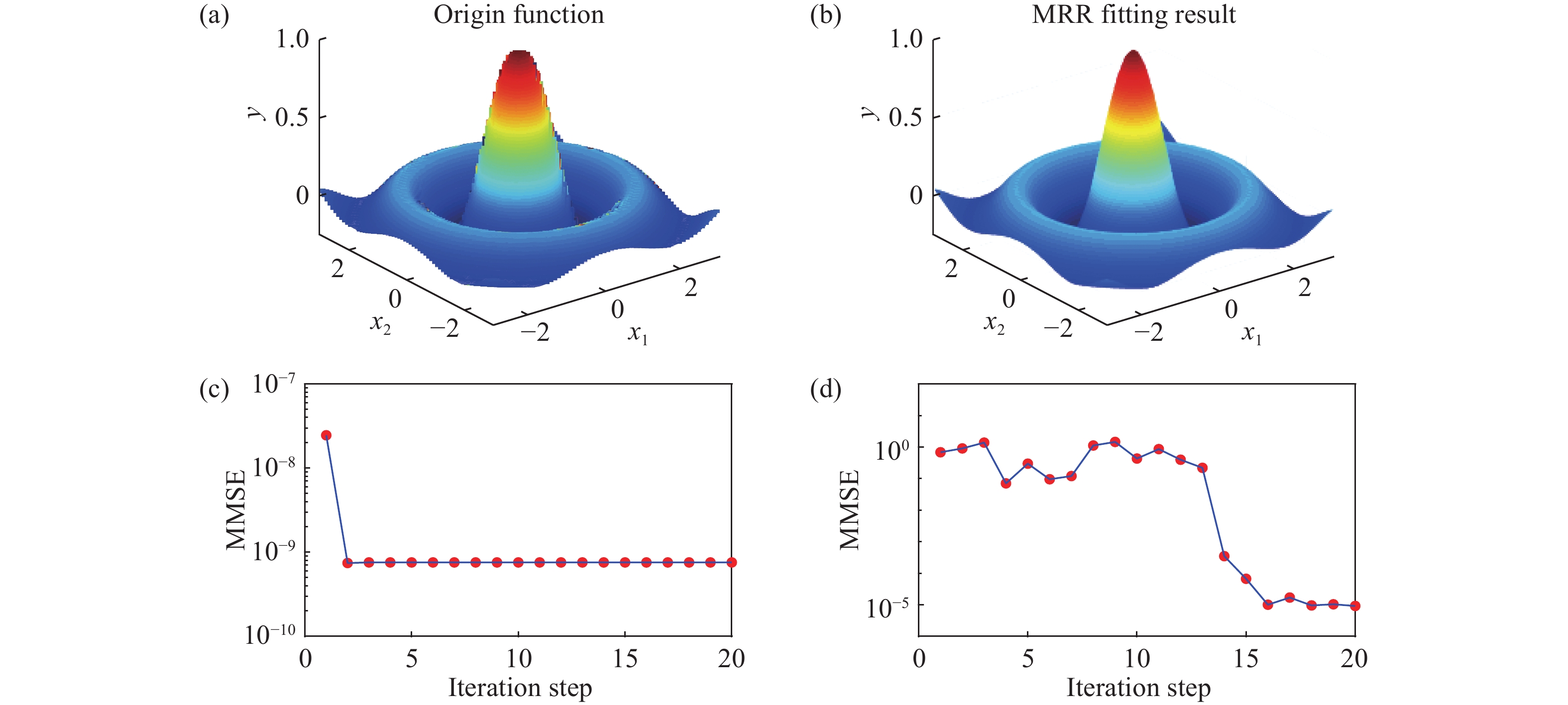
Fig. 1.
(Color online) The original function and MRR fitting function. (a) Original artificial function. (b) Single-pole MRR fitting result. (c) Step NMSEs of single-pole MRR. (d) Step NMSEs of double-pole MRR.
SEMICONDUCTOR DEVICES
Yuxi Hong, Dongsheng Ma and Zuochang Ye
Corresponding author: Zuochang Ye, zuochang@tsinghua.edu.cn
Abstract: Physics equation-based semiconductor device modeling is accurate but time and money consuming. The need for studying new material and devices is increasing so that there has to be an efficient and accurate device modeling method. In this paper, two methods based on multivariate rational regression (MRR) for device modeling are proposed. They are single-pole MRR and double-pole MRR. The two MRR methods are proved to be powerful in nonlinear curve fitting and have good numerical stability. Two methods are compared with OLS and LASSO by fitting the SMIC 40 nm MOS-FET I–V characteristic curve and the normalized mean square error of Single-pole MRR is
Keywords: multivariate rational regression, MRR, semiconductor device modeling, vector fitting
| [1] |
Sheu B J, Scharfetter D L, Ko P K, et al. BSIM: Berkeley short-channel IGFET model for MOS transistors. IEEE J Solid-State Circuits, 1987, 22(4): 558 doi: 10.1109/JSSC.1987.1052773
|
| [2] |
Waldrop M M. The chips are down for Moore’s law. Nature, 2016, 530(7589): 144 doi: 10.1038/530144a
|
| [3] |
Kim S H, Song W, Jung M W, et al. Carbon nanotube and graphene hybrid thin film for transparent electrodes and field effect transistors. Adv Mater, 2014, 26(25): 4247 doi: 10.1002/adma.v26.25
|
| [4] |
Chen B, Zhang P, Ding L, et al. Highly uniform carbon nanotube field-effect transistors and medium scale integrated circuits. Nano Lett, 2016, 16(8): 5120 doi: 10.1021/acs.nanolett.6b02046
|
| [5] |
Grivet-Talocia S, Gustavsen B. Black-box macromodeling and curve fitting, in passive macromodeling: theory and applications. John Wiley & Sons, Inc, 2015
|
| [6] |
Bañuelos-Cabral E S, Gutiérrez-Robles J A, Gustavsen B. Rational fitting techniques for the modeling of electric power components and systems using MATLAB environment. InTech, 2017
|
| [7] |
Grivet-Talocia S, Gustavsen B. Black-box macromodeling and its EMC applications. IEEE Electromagn Compat Mag, 2016, 5(3): 71
|
| [8] |
Bañuelos-Cabral E S, Gutiérrez-Robles J A, Gustavsen B, et al. Enhancing the accuracy of rational function-based models using optimization. Electr Power Syst Res, 2015, 125: 83 doi: 10.1016/j.jpgr.2015.04.001
|
| [9] |
Avouris P, Chen Z H, Perebeinos V. Carbon-based electronics. Nat Nanotechnol, 2017, 2(10): 605
|
| [10] |
Che Y C, Chen H T, Gui H, et al. Review of carbon nanotube nanoeletronics and macroelectronics. Semicond Sci Technol, 2014, 29(7): 073001 doi: 10.1088/0268-1242/29/7/073001
|
| [11] |
Derenskyi V, Gomulya W, Rios J M S, et al. Carbon nanotube network ambipolar field‐effect transistors with 108 on/off ratio. Adv Mater, 2014, 26(34): 5969 doi: 10.1002/adma.201401395
|
| [12] |
Friedman J, Hastie T, Tibshirani R. The elements of statistical learning. New York: Springer, 2001
|
| [13] |
Levy E C. Complex-curve fitting. IRE Trans Autom Control, 1959, 4(1): 37
|
| [14] |
Sanathanan C, Koerner J. Transfer function synthesis as a ratio of two complex polynomials. IEEE Trans Autom Control, 1963, 8(1): 56 doi: 10.1109/TAC.1963.1105517
|
| [15] |
Lawrence P J, Rogers G J. Sequential transfer-function synthesis from measured data. Proceedings of the Institution of Electrical Engineers, 1979, 126(1): 104 doi: 10.1049/piee.1979.0020
|
| [16] |
Whitfield A H. Transfer function synthesis using frequency response data. Int J Control, 1986, 43(5): 1413 doi: 10.1080/00207178608933548
|
| [17] |
Pintelon R, Guillaume P, Rolain Y, et al. Parametric identification of transfer functions in the frequency domain-a survey. IEEE Trans Autom Control, 1994, 39(11): 2245 doi: 10.1109/9.333769
|
| [18] |
Gustavsen B, Semlyen A. Rational approximation of frequency domain responses by vector fitting. IEEE Trans Power Deliv, 1999, 14(3): 1052 doi: 10.1109/61.772353
|
| [19] |
Grivet-Talocia S, Gustavsen B. The vector fitting algorithm, in passive macromodeling: theory and applications. John Wiley & Sons, Inc, 2015
|
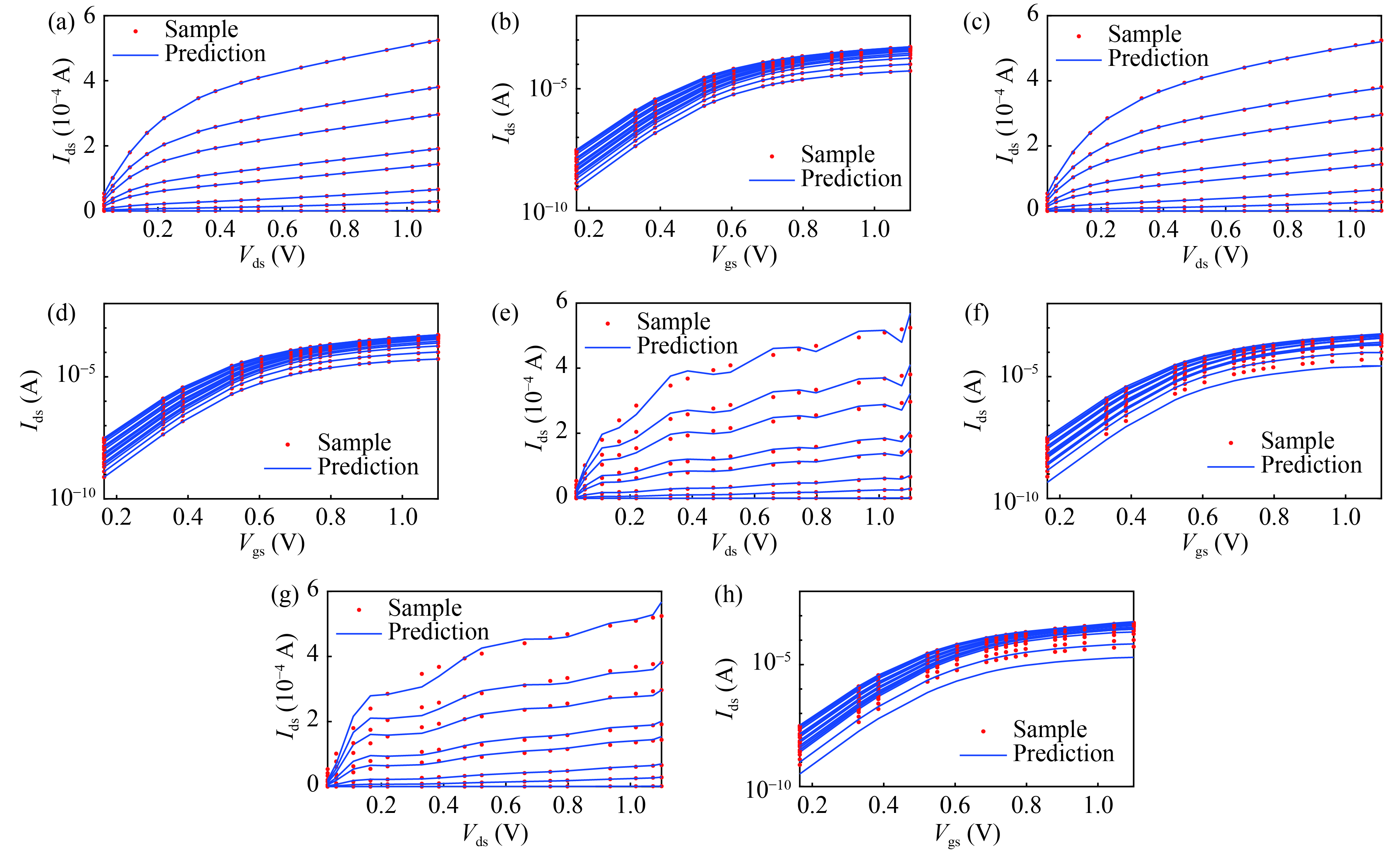
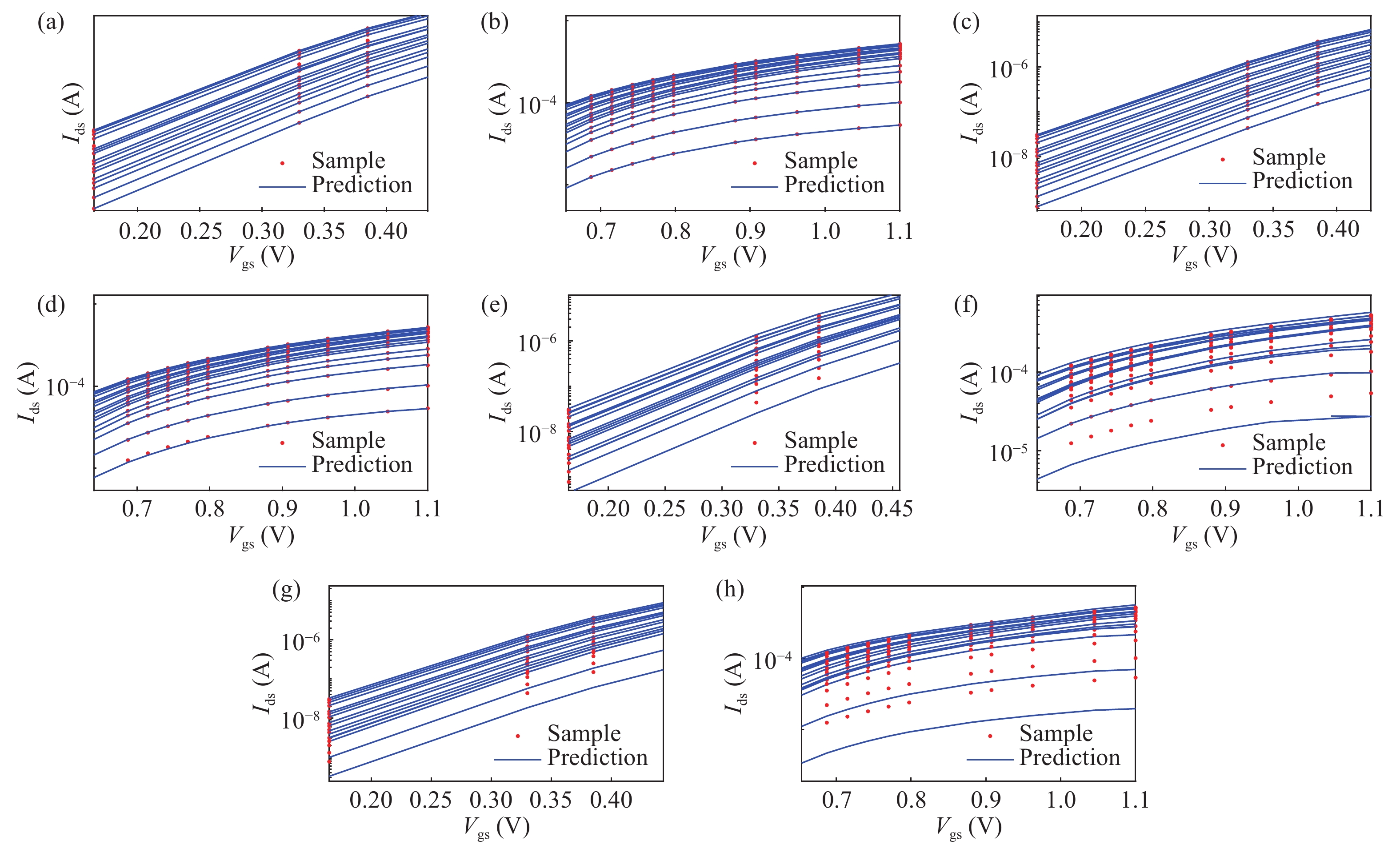
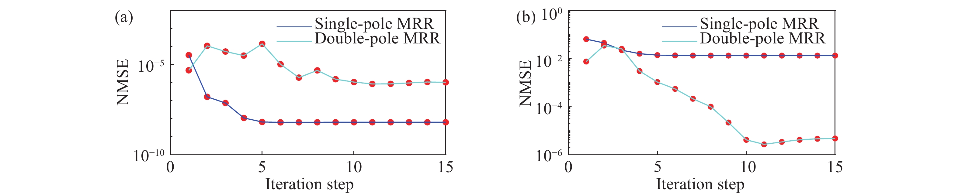
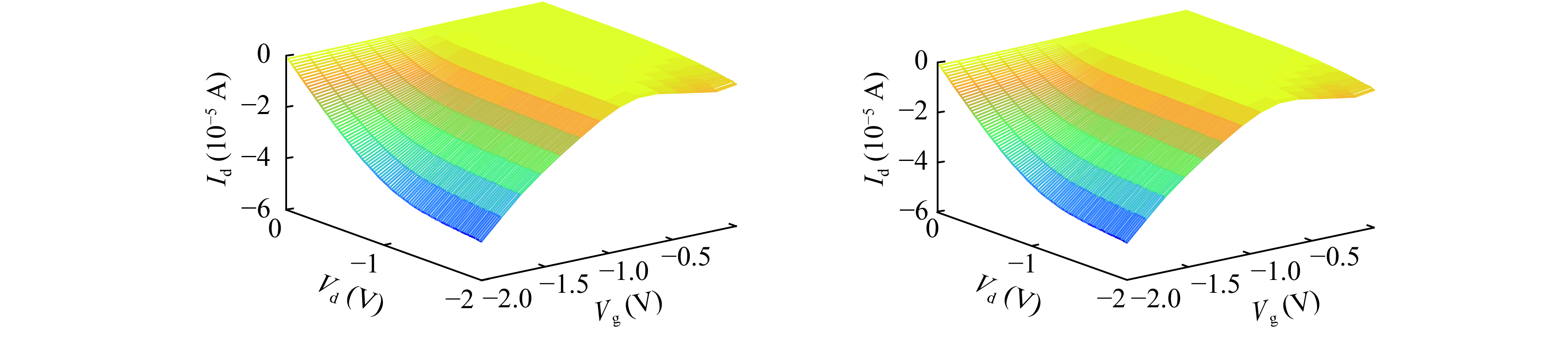
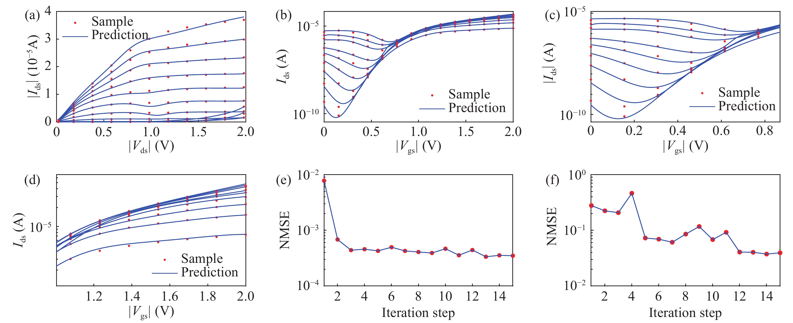
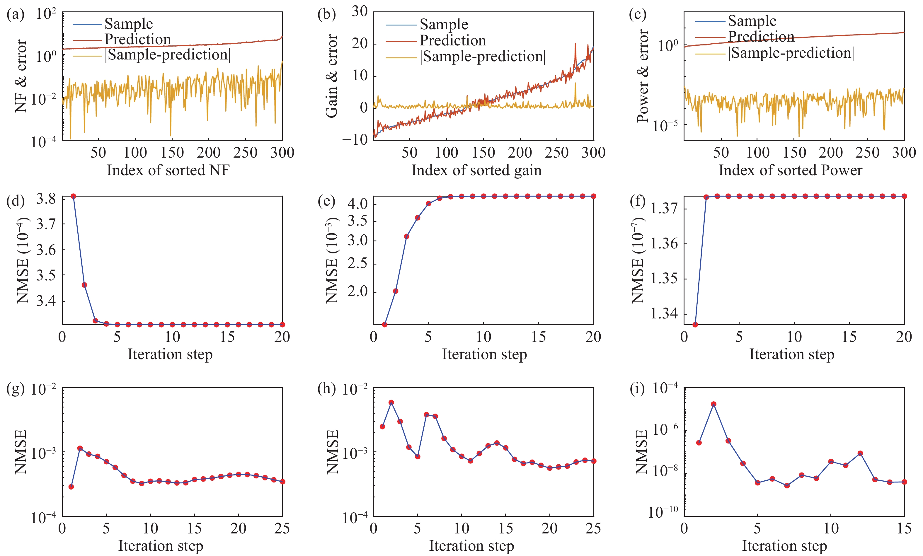
Table 1. NMSE and parameters number results of different algorithms.
| Algorithm | Single-pole MRR
(sextic polynomial) |
Double-pole MRR
(quartic polynomial) |
OLS
(nonic polynomial) |
LASSO
(nonic polynomial) |
| Parameter | 55 | 58 | 55 | 36 |
| NMSE | 3.0157 × 10⁻⁸ | 2.631 × 10⁻⁶ | 4.357 × 10⁻⁴ | 5.082 × 10⁻⁴ |
 DownLoad: CSV
| [1] |
Sheu B J, Scharfetter D L, Ko P K, et al. BSIM: Berkeley short-channel IGFET model for MOS transistors. IEEE J Solid-State Circuits, 1987, 22(4): 558 doi: 10.1109/JSSC.1987.1052773
|
| [2] |
Waldrop M M. The chips are down for Moore’s law. Nature, 2016, 530(7589): 144 doi: 10.1038/530144a
|
| [3] |
Kim S H, Song W, Jung M W, et al. Carbon nanotube and graphene hybrid thin film for transparent electrodes and field effect transistors. Adv Mater, 2014, 26(25): 4247 doi: 10.1002/adma.v26.25
|
| [4] |
Chen B, Zhang P, Ding L, et al. Highly uniform carbon nanotube field-effect transistors and medium scale integrated circuits. Nano Lett, 2016, 16(8): 5120 doi: 10.1021/acs.nanolett.6b02046
|
| [5] |
Grivet-Talocia S, Gustavsen B. Black-box macromodeling and curve fitting, in passive macromodeling: theory and applications. John Wiley & Sons, Inc, 2015
|
| [6] |
Bañuelos-Cabral E S, Gutiérrez-Robles J A, Gustavsen B. Rational fitting techniques for the modeling of electric power components and systems using MATLAB environment. InTech, 2017
|
| [7] |
Grivet-Talocia S, Gustavsen B. Black-box macromodeling and its EMC applications. IEEE Electromagn Compat Mag, 2016, 5(3): 71
|
| [8] |
Bañuelos-Cabral E S, Gutiérrez-Robles J A, Gustavsen B, et al. Enhancing the accuracy of rational function-based models using optimization. Electr Power Syst Res, 2015, 125: 83 doi: 10.1016/j.jpgr.2015.04.001
|
| [9] |
Avouris P, Chen Z H, Perebeinos V. Carbon-based electronics. Nat Nanotechnol, 2017, 2(10): 605
|
| [10] |
Che Y C, Chen H T, Gui H, et al. Review of carbon nanotube nanoeletronics and macroelectronics. Semicond Sci Technol, 2014, 29(7): 073001 doi: 10.1088/0268-1242/29/7/073001
|
| [11] |
Derenskyi V, Gomulya W, Rios J M S, et al. Carbon nanotube network ambipolar field‐effect transistors with 108 on/off ratio. Adv Mater, 2014, 26(34): 5969 doi: 10.1002/adma.201401395
|
| [12] |
Friedman J, Hastie T, Tibshirani R. The elements of statistical learning. New York: Springer, 2001
|
| [13] |
Levy E C. Complex-curve fitting. IRE Trans Autom Control, 1959, 4(1): 37
|
| [14] |
Sanathanan C, Koerner J. Transfer function synthesis as a ratio of two complex polynomials. IEEE Trans Autom Control, 1963, 8(1): 56 doi: 10.1109/TAC.1963.1105517
|
| [15] |
Lawrence P J, Rogers G J. Sequential transfer-function synthesis from measured data. Proceedings of the Institution of Electrical Engineers, 1979, 126(1): 104 doi: 10.1049/piee.1979.0020
|
| [16] |
Whitfield A H. Transfer function synthesis using frequency response data. Int J Control, 1986, 43(5): 1413 doi: 10.1080/00207178608933548
|
| [17] |
Pintelon R, Guillaume P, Rolain Y, et al. Parametric identification of transfer functions in the frequency domain-a survey. IEEE Trans Autom Control, 1994, 39(11): 2245 doi: 10.1109/9.333769
|
| [18] |
Gustavsen B, Semlyen A. Rational approximation of frequency domain responses by vector fitting. IEEE Trans Power Deliv, 1999, 14(3): 1052 doi: 10.1109/61.772353
|
| [19] |
Grivet-Talocia S, Gustavsen B. The vector fitting algorithm, in passive macromodeling: theory and applications. John Wiley & Sons, Inc, 2015
|


Article views: 5113 Times PDF downloads: 72 Times Cited by: 0 Times
Received: 07 January 2018 Revised: 12 March 2018 Online: Uncorrected proof: 25 April 2018Accepted Manuscript: 26 April 2018Published: 01 September 2018
| Citation: |
Yuxi Hong, Dongsheng Ma, Zuochang Ye. Multivariate rational regression and its application in semiconductor device modeling[J]. Journal of Semiconductors, 2018, 39(9): 094010. doi: 10.1088/1674-4926/39/9/094010
****
Y X Hong, D S Ma, Z C Ye, Multivariate rational regression and its application in semiconductor device modeling[J]. J. Semicond., 2018, 39(9): 094010. doi: 10.1088/1674-4926/39/9/094010.

|
| [1] |
Sheu B J, Scharfetter D L, Ko P K, et al. BSIM: Berkeley short-channel IGFET model for MOS transistors. IEEE J Solid-State Circuits, 1987, 22(4): 558 doi: 10.1109/JSSC.1987.1052773
|
| [2] |
Waldrop M M. The chips are down for Moore’s law. Nature, 2016, 530(7589): 144 doi: 10.1038/530144a
|
| [3] |
Kim S H, Song W, Jung M W, et al. Carbon nanotube and graphene hybrid thin film for transparent electrodes and field effect transistors. Adv Mater, 2014, 26(25): 4247 doi: 10.1002/adma.v26.25
|
| [4] |
Chen B, Zhang P, Ding L, et al. Highly uniform carbon nanotube field-effect transistors and medium scale integrated circuits. Nano Lett, 2016, 16(8): 5120 doi: 10.1021/acs.nanolett.6b02046
|
| [5] |
Grivet-Talocia S, Gustavsen B. Black-box macromodeling and curve fitting, in passive macromodeling: theory and applications. John Wiley & Sons, Inc, 2015
|
| [6] |
Bañuelos-Cabral E S, Gutiérrez-Robles J A, Gustavsen B. Rational fitting techniques for the modeling of electric power components and systems using MATLAB environment. InTech, 2017
|
| [7] |
Grivet-Talocia S, Gustavsen B. Black-box macromodeling and its EMC applications. IEEE Electromagn Compat Mag, 2016, 5(3): 71
|
| [8] |
Bañuelos-Cabral E S, Gutiérrez-Robles J A, Gustavsen B, et al. Enhancing the accuracy of rational function-based models using optimization. Electr Power Syst Res, 2015, 125: 83 doi: 10.1016/j.jpgr.2015.04.001
|
| [9] |
Avouris P, Chen Z H, Perebeinos V. Carbon-based electronics. Nat Nanotechnol, 2017, 2(10): 605
|
| [10] |
Che Y C, Chen H T, Gui H, et al. Review of carbon nanotube nanoeletronics and macroelectronics. Semicond Sci Technol, 2014, 29(7): 073001 doi: 10.1088/0268-1242/29/7/073001
|
| [11] |
Derenskyi V, Gomulya W, Rios J M S, et al. Carbon nanotube network ambipolar field‐effect transistors with 108 on/off ratio. Adv Mater, 2014, 26(34): 5969 doi: 10.1002/adma.201401395
|
| [12] |
Friedman J, Hastie T, Tibshirani R. The elements of statistical learning. New York: Springer, 2001
|
| [13] |
Levy E C. Complex-curve fitting. IRE Trans Autom Control, 1959, 4(1): 37
|
| [14] |
Sanathanan C, Koerner J. Transfer function synthesis as a ratio of two complex polynomials. IEEE Trans Autom Control, 1963, 8(1): 56 doi: 10.1109/TAC.1963.1105517
|
| [15] |
Lawrence P J, Rogers G J. Sequential transfer-function synthesis from measured data. Proceedings of the Institution of Electrical Engineers, 1979, 126(1): 104 doi: 10.1049/piee.1979.0020
|
| [16] |
Whitfield A H. Transfer function synthesis using frequency response data. Int J Control, 1986, 43(5): 1413 doi: 10.1080/00207178608933548
|
| [17] |
Pintelon R, Guillaume P, Rolain Y, et al. Parametric identification of transfer functions in the frequency domain-a survey. IEEE Trans Autom Control, 1994, 39(11): 2245 doi: 10.1109/9.333769
|
| [18] |
Gustavsen B, Semlyen A. Rational approximation of frequency domain responses by vector fitting. IEEE Trans Power Deliv, 1999, 14(3): 1052 doi: 10.1109/61.772353
|
| [19] |
Grivet-Talocia S, Gustavsen B. The vector fitting algorithm, in passive macromodeling: theory and applications. John Wiley & Sons, Inc, 2015
|

 WeChat ID
Journal of Semiconductors © 2017 All Rights Reserved 京ICP备05085259号-2